Convergence of Quantum Neural Networks

Introduction

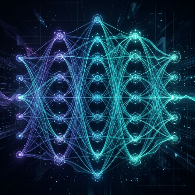
Quantum Neural Networks (QNNs) — more precisely called Parameterized Quantum Circuits (PQCs) — are the quantum analogue of classical neural networks. Instead of tunable weight matrices, they consist of sequences of quantum gates whose rotation angles $\boldsymbol{\theta} \in \mathbb{R}^p$ are optimized to minimize a cost function.

The central question this article addresses is deceptively simple: do QNNs converge during training, and under what conditions?

This is not merely an academic question. The practical viability of near-term quantum machine learning depends entirely on whether gradient-based optimization of these circuits is tractable. As we will show, there are fundamental theoretical barriers — most notably the barren plateau phenomenon — that make this a genuinely hard problem, and an active area of research.

We will derive everything from first principles. No hand-waving.

---

1. The Parameterized Quantum Circuit Model

1.1 Circuit Structure

A PQC acting on $n$ qubits is a unitary operator of the form:

where:

• $W_l$ are fixed (non-parameterized) unitary gates such as CNOT entangling layers
• $U_l(\theta_l) = e^{-i \theta_l H_l / 2}$ are parameterized rotation gates generated by Hermitian operators $H_l$ (typically Pauli operators $X$, $Y$, or $Z$)
• $L$ is the total number of parameterized layers

The circuit acts on an initial state $|0\rangle^{\otimes n}$ to produce:

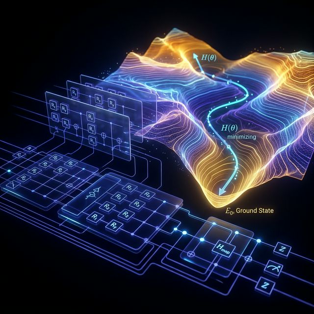
1.2 The Cost Function

Training a QNN means minimizing a cost function $C(\boldsymbol{\theta})$. For most variational tasks this takes the form:

where $\hat{O}$ is an observable (Hermitian operator) encoding the task objective, and $\rho_0 = |0\rangle\langle 0|^{\otimes n}$ is the initial state density matrix.

For supervised learning, the cost typically involves a training dataset $\{(x_i, y_i)\}$ and encodes each input via a data-embedding unitary $S(x_i)$:

where $\ell$ is a loss function (e.g., squared error or cross-entropy) and $|\psi_i(\boldsymbol{\theta})\rangle = U(\boldsymbol{\theta})S(x_i)|0\rangle^{\otimes n}$.

---

2. Gradient Computation: The Parameter-Shift Rule

To optimize $C(\boldsymbol{\theta})$ via gradient descent, we need $\partial C / \partial \theta_k$ for each parameter. Unlike classical automatic differentiation, quantum gradients must be computed on hardware using the parameter-shift rule [Mitarai et al., 2018; Schuld et al., 2019].

2.1 Derivation

Since each parameterized gate has the form $U_k(\theta_k) = e^{-i\theta_k H_k / 2}$ where $H_k$ has eigenvalues $\pm 1$ (true for all single-qubit Pauli rotations), the cost function is sinusoidal in each parameter:

$$C(\theta_k) = a \cos(\theta_k) + b \sin(\theta_k) + c$$

for some constants $a$, $b$, $c$ that depend on all other parameters. This means the exact gradient is:

$$\frac{\partial C}{\partial \theta_k} = \frac{C\!\left(\theta_k + \frac{\pi}{2}\right) - C\!\left(\theta_k - \frac{\pi}{2}\right)}{2}$$

This is the parameter-shift rule. It requires exactly two circuit evaluations per parameter to compute the exact gradient — no finite differences, no approximation. For $p$ parameters, full gradient computation costs $2p$ circuit evaluations per optimization step.

2.2 Gradient Descent Update

Standard gradient descent updates are:

$$\boldsymbol{\theta}^{(t+1)} = \boldsymbol{\theta}^{(t)} - \eta \nabla_{\boldsymbol{\theta}} C\!\left(\boldsymbol{\theta}^{(t)}\right)$$

where $\eta > 0$ is the learning rate. Variants like Adam and SPSA are also commonly used in practice.

---

3. The Barren Plateau Problem

Here is where convergence theory becomes deeply problematic. In 2018, McClean et al. proved a theorem that fundamentally challenges the trainability of large QNNs [McClean et al., 2018, Nature Communications].

3.1 The Theorem (McClean et al., 2018)

Theorem. Consider a PQC $U(\boldsymbol{\theta})$ drawn from a unitary 2-design (a circuit expressive enough to approximate the Haar measure on the unitary group $U(2^n)$). For any partial derivative and any observable $\hat{O}$ with $\text{Tr}[\hat{O}] = 0$:

$$\mathbb{E}_{\boldsymbol{\theta}}\left[\frac{\partial C}{\partial \theta_k}\right] = 0$$ $$\text{Var}_{\boldsymbol{\theta}}\left[\frac{\partial C}{\partial \theta_k}\right] \leq \frac{1}{2^n} \cdot f(L)$$

where $f(L)$ is a function of depth $L$ that decreases exponentially in $n$ for deep circuits.

What this means in plain terms: As the number of qubits $n$ grows, the gradient variance shrinks exponentially. The gradient landscape becomes exponentially flat — a barren plateau — and gradient-based optimizers cannot determine which direction to move. The gradients are essentially zero everywhere, to within measurement precision.

3.2 Intuition via the Haar Measure

The Haar measure on $U(2^n)$ is the uniform distribution over all $2^n \times 2^n$ unitary matrices. When a circuit approximates this distribution (which deep, expressive circuits tend to do), the output state $|\psi(\boldsymbol{\theta})\rangle$ is effectively a uniformly random point on the $2^{2^n}$-dimensional complex unit sphere.

The observable $\hat{O}$ projected onto this sphere has expectation near zero for almost all states (by the concentration of measure phenomenon), and the variance of this expectation over random states is $O(2^{-n})$.

This is not a bug in the optimization algorithm — it is a geometric property of high-dimensional quantum state space.

3.3 Depth Dependence

For local observables (those acting on only $O(1)$ qubits), Cerezo et al. [2021, Nature Communications] showed that shallow circuits (depth $O(\log n)$) can avoid barren plateaus. The variance scaling becomes:

$$\text{Var}\left[\frac{\partial C}{\partial \theta_k}\right] = \Omega\!\left(\frac{1}{\text{poly}(n)}\right) \quad \text{(shallow, local observable)}$$ $$\text{Var}\left[\frac{\partial C}{\partial \theta_k}\right] = O\!\left(\frac{1}{b^n}\right),\; b > 1 \quad \text{(deep, global observable)}$$

This gives a concrete design guideline: use shallow circuits with local cost functions to maintain trainability on NISQ hardware.

---

4. Convergence Conditions

Given the barren plateau issue, under what conditions can QNN training provably converge?

4.1 Overparameterization Regime

Larocca et al. [2023, Nature Computational Science] and Fontana et al. [2023] established that QNNs enter an overparameterized regime when the number of parameters $p$ exceeds the dimension of the Dynamical Lie Algebra (DLA) of the circuit.

The DLA $\mathfrak{g}$ is the Lie algebra generated by the Hamiltonians $\{H_l\}$ under commutators:

$$\mathfrak{g} = \text{span}_{\mathbb{R}}\left\{H_l,\, [H_j, H_k],\, [H_j, [H_k, H_l]],\, \ldots \right\}$$

Theorem (Overparameterization, informal). If $p \geq \dim(\mathfrak{g})$, then the optimization landscape of $C(\boldsymbol{\theta})$ has no spurious local minima — every local minimum is a global minimum.

This is the QNN analogue of classical neural network overparameterization results. However, the DLA dimension grows exponentially with $n$ in general, so overparameterization at scale remains computationally expensive.

4.2 Convergence Rate for Convex Cost Landscapes

In the overparameterized regime, if $C(\boldsymbol{\theta})$ is locally convex around the initialization, gradient descent with step size $\eta \leq 1/L_C$ (where $L_C$ is the Lipschitz constant of $\nabla C$) converges at rate:

$$C(\boldsymbol{\theta}^{(T)}) - C^* \leq \frac{\|\boldsymbol{\theta}^{(0)} - \boldsymbol{\theta}^*\|^2}{2\eta T}$$

This is standard convex optimization, $O(1/T)$ convergence. But this guarantee only holds when barren plateaus are absent.

4.3 The Noise Barrier

On real NISQ hardware, there is an additional convergence barrier from decoherence and gate noise. Wang et al. [2021, Nature Communications] showed that hardware noise itself induces an effect analogous to barren plateaus:

$$\left|\frac{\partial C_{\text{noisy}}}{\partial \theta_k}\right| \leq c \cdot \lambda^d$$

where $\lambda < 1$ is related to the gate error rate and $d$ is the circuit depth. As depth increases to gain expressibility, noise exponentially suppresses the cost gradient signal. This creates a fundamental tension: expressibility requires depth, but depth kills gradients via noise.

---

5. Mitigation Strategies

The research community has proposed several approaches to escape barren plateaus:

1. Local cost functions [Cerezo et al., 2021]: Instead of global observables like $\hat{O} = |0\rangle\langle 0|^{\otimes n}$, use sums of local terms: $\hat{O} = \sum_i \hat{O}_i$ where each $\hat{O}_i$ acts on $O(1)$ qubits. This preserves polynomial gradient variance for shallow circuits.

2. Layer-wise training [Skolik et al., 2021, Quantum Machine Intelligence]: Train the circuit one layer at a time, fixing previously trained layers. This limits the effective dimensionality of each training problem.

3. Structured ansätze: Use hardware-efficient ansätze with limited expressibility by design — restricting the DLA to prevent approximation of a unitary 2-design. Examples include the QAOA ansatz and chemically-inspired ansätze for quantum chemistry.

4. Quantum natural gradient [Stokes et al., 2020, Quantum]: Replace the Euclidean gradient with the quantum geometric tensor (Fubini-Study metric):

$$\boldsymbol{\theta}^{(t+1)} = \boldsymbol{\theta}^{(t)} - \eta \, F^{+}(\boldsymbol{\theta}^{(t)}) \nabla C(\boldsymbol{\theta}^{(t)})$$

where $F^{+}$ is the pseudoinverse of the quantum Fisher information matrix. This corrects for the non-Euclidean geometry of quantum state space and can significantly accelerate convergence.

---

6. Current State (2024–2025)

As of the most recent literature, the honest assessment is:

• Small-scale QNNs ($n \leq 10$ qubits, shallow depth) can be trained reliably on simulators and current hardware with appropriate cost function design
• Medium-scale systems ($10 < n \leq 100$ qubits) face severe barren plateau and noise barriers that no mitigation strategy fully resolves at this time
• Fault-tolerant QNNs remain a long-term prospect, contingent on advances in quantum error correction

The field is not stagnant — new results on equivariant QNNs [Larocca et al., 2022] and quantum kernel methods offer alternative paths that sidestep some trainability issues entirely.

---

Conclusion

QNN convergence is theoretically possible under specific conditions — overparameterized regimes, shallow circuits, local observables — but is fundamentally limited by the barren plateau phenomenon, which is not an artifact of poor implementation but a mathematical consequence of high-dimensional quantum geometry.

The honest position in 2025 is that training large QNNs on practical problems remains an open problem. Progress is being made, but anyone claiming otherwise should be asked to show the gradient variances.

---

References

1. McClean, J. R., Boixo, S., Smelyanskiy, V. N., Babbush, R., & Neven, H. (2018). Barren plateaus in quantum neural network training landscapes. Nature Communications, 9(1), 4812. https://doi.org/10.1038/s41467-018-07090-4

2. Mitarai, K., Negoro, M., Kitagawa, M., & Fujii, K. (2018). Quantum circuit learning. Physical Review A, 98(3), 032309. https://doi.org/10.1103/PhysRevA.98.032309

3. Schuld, M., Bergholm, V., Gogolin, C., Izaac, J., & Killoran, N. (2019). Evaluating analytic gradients on quantum hardware. Physical Review A, 99(3), 032331. https://doi.org/10.1103/PhysRevA.99.032331

4. Cerezo, M., Sone, A., Volkoff, T., Cincio, L., & Coles, P. J. (2021). Cost function dependent barren plateaus in shallow parametrized quantum circuits. Nature Communications, 12(1), 1791. https://doi.org/10.1038/s41467-021-21728-w

5. Larocca, M., Czarnik, P., Sharma, K., Muraleedharan, G., Coles, P. J., & Dankert, M. (2023). Diagnosing barren plateaus with tools from quantum optimal control. Nature Computational Science, 3, 1–9. https://doi.org/10.1038/s43588-023-00497-6

6. Wang, S., Fontana, E., Cerezo, M., Sharma, K., Sone, A., Cincio, L., & Coles, P. J. (2021). Noise-induced barren plateaus in variational quantum algorithms. Nature Communications, 12(1), 6961. https://doi.org/10.1038/s41467-021-27045-6

7. Stokes, J., Izaac, J., Killoran, N., & Carleo, G. (2020). Quantum natural gradient. Quantum, 4, 269. https://doi.org/10.22331/q-2020-05-25-269

8. Skolik, A., McClean, J. R., Mohseni, M., van der Smagt, P., & Leib, M. (2021). Layerwise learning for quantum neural networks. Quantum Machine Intelligence, 3(1), 5. https://doi.org/10.1007/s42484-020-00036-4

---